If you've just started learning Data Structures and Algorithms, you've probably heard people say things like "This algorithm is O(n)" or "That solution is O(log n)." At first, it sounds confusing, but don't worry—it’s actually much simpler than it looks.

Think about it this way. Imagine you're planning a road trip. Sometimes the road is completely empty and you reach your destination quickly. Sometimes there's normal traffic, and other times you're stuck in a huge traffic jam with roadblocks and construction everywhere. The route is the same, but the time it takes changes depending on the situation.

That's exactly how algorithms work.

Sometimes they finish very quickly, sometimes they take an average amount of time, and sometimes they take the maximum possible time. This idea is what Time Complexity is all about.

Along with time, algorithms also use memory. Some algorithms are extremely fast but need extra memory, while others use very little memory but run slower. That's where Space Complexity comes in.

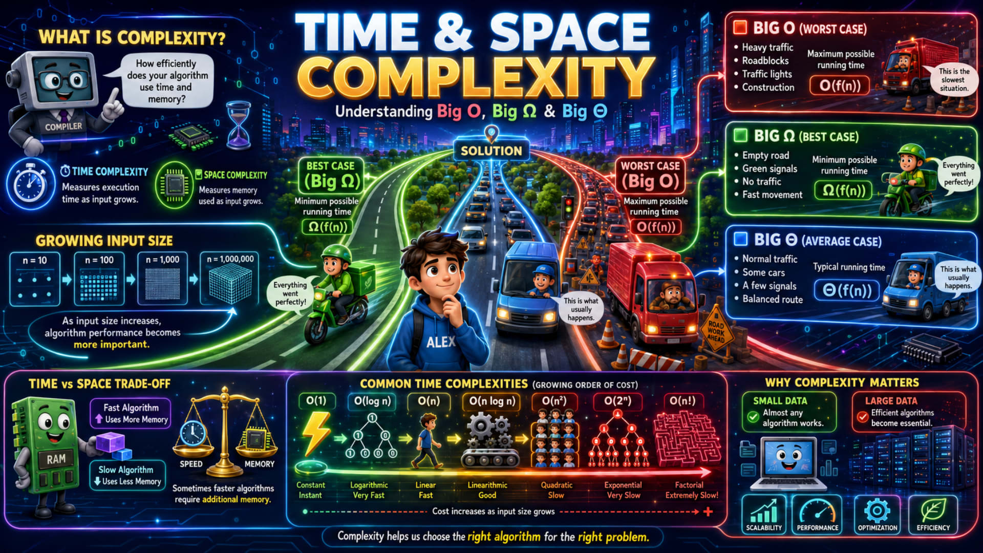
Let's understand everything shown in the infographic one by one.

What is Complexity?

The slide starts with a simple question:

How efficiently does your algorithm use time and memory?

Whenever we write a program, we usually care about two things:

• How long it takes to finish.

• How much memory it consumes.

These two measurements together are called the complexity of an algorithm.

Instead of checking the exact running time in seconds, we study how the algorithm behaves when the input becomes larger.

For example, suppose your program sorts 10 numbers in one second.

Now imagine sorting:

• 100 numbers

• 1,000 numbers

• 1 million numbers

Will it still finish in one second?

Of course not.

Different algorithms grow differently as the input size increases, and that's exactly what complexity measures.

Time Complexity

The infographic defines Time Complexity as:

Measures execution time as input grows.

Notice something important here.

It does not mean measuring time using a stopwatch.

If you run the same Java program:

• on your laptop,

• on a gaming PC,

• on a cloud server,

the execution time will be different because the hardware is different.

Instead, we measure how the number of operations increases as the input size (n) increases.

Suppose we have this Java code:

for(int i = 0; i < n; i++){
    System.out.println(i);
}

If:

• n = 5 → loop runs 5 times

• n = 100 → loop runs 100 times

• n = 1,000 → loop runs 1,000 times

The work grows directly with n, so we say the algorithm has O(n) time complexity.

Space Complexity

The infographic also explains:

Measures memory used as input grows.

Every program stores data somewhere.

For example,

int[] arr = new int[n];

If:

• n = 10

we store 10 integers.

If:

• n = 1000

we store 1000 integers.

The memory usage grows with the input size.

That's why its space complexity is also O(n).

If an algorithm only uses a few variables regardless of input size, then its space complexity is O(1).

Growing Input Size

The slide beautifully shows input sizes increasing:

• n = 10

• n = 100

• n = 1,000

• n = 1,000,000

This is the most important idea in DSA.

Small inputs don't really tell us whether an algorithm is good or bad.

Even an inefficient algorithm may look fast when n = 10.

The real difference appears when n becomes huge.

Imagine searching for a name:

In a notebook containing:

• 10 names

• 100 names

• 1 million names

An inefficient search method may take forever for the third case.

That's why complexity focuses on large inputs, not tiny ones.

Understanding Big O, Big Ω and Big Θ Using the Road Example

This infographic uses one of the best real-life analogies.

Alex wants to reach the solution, but the road conditions keep changing.

Let's understand each route.

Big Ω (Best Case)

The green road represents the best possible situation.

The slide mentions:

• Empty road

• Green signals

• No traffic

• Fast movement

Everything goes perfectly.

The delivery rider reaches the destination as quickly as possible.

This represents the minimum possible running time.

Mathematically,

Big Ω (Omega) tells us the best-case complexity.

For example, consider searching in a sorted array.

If the element you're searching for is already at the first position,

you find it immediately.

Only one comparison happens.

That's the best-case scenario.

Big Θ (Average Case)

Now look at the blue road.

This is what usually happens in real life.

The infographic mentions:

• Normal traffic

• Some cars

• A few signals

• Balanced route

Sometimes you stop.

Sometimes you move.

Overall, the journey is neither extremely fast nor extremely slow.

This represents the typical running time.

That's exactly what Big Θ (Theta) represents.

Most of the time, algorithms behave close to this.

Big O (Worst Case)

Finally, we have the red road.

The infographic shows:

• Heavy traffic

• Roadblocks

• Construction

• Traffic lights

The truck barely moves.

Everything that could go wrong has gone wrong.

This is the maximum possible running time.

This is called Big O.

When interviewers ask,

"What's the time complexity?"

They are almost always asking for the Big O complexity, because it guarantees that the algorithm will never perform worse than this limit.

Why Do We Usually Focus on Big O?

You might wonder,

"If there are three notations, why does everyone talk about Big O?"

Because software engineers want guarantees.

Suppose your algorithm usually finishes in one second.

But once in a while it takes two minutes.

That could crash an application or make users leave.

Big O tells us the maximum time an algorithm may take.

That's why it is the most commonly used notation.

Time vs Space Trade-Off

Another interesting concept shown in the infographic is the Time vs Space Trade-Off.

The RAM character explains it perfectly.

Sometimes,

a fast algorithm uses more memory.

Other times,

a slower algorithm uses less memory.

Think of Google Maps.

It stores a huge amount of map data in memory so it can calculate routes very quickly.

More memory.

Less time.

Now imagine calculating every route from scratch every single time.

Less memory.

More time.

There is always a balance.

As the scale in the infographic shows, sometimes we sacrifice memory for speed, and sometimes we sacrifice speed to save memory.

There is no universal "best" choice—it depends on the problem and the available resources.

Common Time Complexities

The infographic also shows the most common time complexities from fastest to slowest.

Let's understand each one.

O(1) — Constant Time

The work never changes.

Whether there are 10 elements or 10 million elements,

the algorithm performs the same amount of work.

Example:

int first = arr[0];

Accessing the first element always takes one operation.

O(log n) — Logarithmic Time

Very efficient.

With every step, the search space becomes roughly half.

Binary Search is the classic example.

Searching in:

• 1,000 elements

• 1 million elements

still requires surprisingly few comparisons.

O(n) — Linear Time

The work grows directly with input size.

Example:

Scanning every element in an array.

If there are 100 elements,

100 checks.

If there are 1,000 elements,

1,000 checks.

O(n log n)

One of the best complexities for sorting.

Algorithms like Merge Sort and Heap Sort belong here.

It is slightly slower than O(n) but much better than quadratic algorithms.

O(n²)

Usually appears with nested loops.

Example:

for(int i=0;i<n;i++){
    for(int j=0;j<n;j++){
        // work
    }
}

Every element is compared with every other element.

Performance drops quickly as input grows.

O(2ⁿ)

Exponential complexity.

Each increase in input size doubles the work.

Common in brute-force recursive solutions where every choice branches into multiple new choices.

These algorithms become impractical even for moderately large inputs.

O(n!)

The slowest among the common complexities shown.

Factorial complexity appears in problems where every possible arrangement or permutation must be explored.

Even small input sizes can result in an enormous number of operations, making such algorithms suitable only for very small datasets.

Why Complexity Matters

The infographic ends with an important message.

For small datasets, almost any algorithm works reasonably well because the amount of data is limited.

But as data grows into thousands, millions, or even billions of elements, choosing the right algorithm becomes critical.

Efficient algorithms help with:

• Better scalability

• Faster performance

• Lower resource usage

• Improved user experience

That's why companies like Google, Amazon, Meta, and Microsoft care so much about algorithm efficiency. Even a small improvement in complexity can save massive amounts of processing time and hardware resources when handling millions of users.

A Few Important Things to Know

There are a few additional concepts that beginners should know while learning complexity analysis:

• Ignore constants: O(2n) is simplified to O(n) because constants don't matter as the input becomes very large.

• Ignore lower-order terms: O(n² + n + 5) becomes O(n²) since the highest-growing term dominates.

• Best, average, and worst case depend on the input: The same algorithm can behave differently for different inputs.

• Time and space are analyzed independently: An algorithm can have excellent time complexity but poor space complexity, or vice versa.

These simplification rules make it easier to compare algorithms based on how they scale, rather than getting distracted by small implementation details.

Conclusion

Time and Space Complexity help us predict how an algorithm will behave as the input size grows. Instead of measuring execution time on a specific computer, complexity analysis focuses on how the number of operations and memory usage increase with larger inputs. The road analogy from the infographic makes this easy to remember: Big Ω is the smooth, empty road representing the best case, Big Θ is the normal traffic representing the average case, and Big O is the worst traffic jam representing the maximum possible running time.

As you continue learning Data Structures and Algorithms, you'll notice that almost every algorithm is compared using these complexity notations. Understanding them early will make topics like searching, sorting, recursion, trees, graphs, and dynamic programming much easier to grasp.

Quick Revision